Abstract
This paper asks a simple question with a less-simple answer: does adding more holdings to a portfolio actually reduce its risk, or does what matters is how those holdings move relative to one another? We build three portfolios from six ETFs spanning US equities, UK equities, US technology equities, US government bonds, gold, and emerging-market equities (SPY, EWU, QQQ, IEF, GLD, EEM; 1 Jan 2017 – 31 Aug 2026), and decompose each portfolio's volatility exactly via σ²ₚ = wᵀΣw. Doubling the number of equity holdings (2 → 4) cuts volatility by only 1.7 percentage points, while adding a single low-correlation, cross-asset holding (4 → 5) cuts it by a further 4.5 points. We then split the sample into three regimes — the 2020 COVID shock, the 2022 rate-hike shock, and the 2023–25 calm market — and show that equity correlations rise in both crises, but the equity–bond relationship does the opposite of what a single "diversification breaks down in a crisis" story would predict: it goes more negative in 2020 (a growth shock) and flips positive in 2022 (an inflation shock). The number of assets held is a weak proxy for diversification; the correlation structure — and the type of shock — is what actually governs it.
Research Question
Conventional wisdom treats diversification and holding count as roughly interchangeable: more positions, less risk. This report tests that assumption directly by asking:
How do correlation and asset allocation affect the volatility of a portfolio?
We do not set out to prove that diversification works — we set out to measure what actually drives it: is it the number of assets held, or the statistical relationship between them? A concentrated two-asset portfolio, a four-asset "diversified" equity portfolio, and a five-asset cross-asset portfolio are constructed from identical building blocks and compared on that basis.
Methodology
For a price series Pₜ, the log return is rₜ = ln(Pₜ / Pₜ₋₁). Annualised return and volatility scale the periodic mean and standard deviation by the number of periods per year, k (here k = 12 for monthly data). Risk-adjusted return is measured by the Sharpe ratio, S = (Rₚ − R𝒻) / σₚ, where R𝒻 is the risk-free rate — proxied here at approximately 2.0%, backed out from the average 3-month T-bill yield over the sample window. Maximum drawdown is the worst peak-to-trough decline in cumulative value, and beta measures an asset's sensitivity to the broad market (m = SPY): βᵢ = Cov(Rᵢ, Rₘ) / Var(Rₘ) = ρᵢ,ₘ (σᵢ / σₘ).
Sample period: 1 January 2017 – 31 August 2026 (approx. 9.7 years) | Frequency: Monthly total returns, dividends reinvested | Data source: Portfolio Visualizer's historical return-and-risk engine
ETFs were used instead of individual stocks so that each series represents a whole asset class rather than company-specific risk. Real historical statistics were sourced through Portfolio Visualizer's own calculation engine rather than re-derived from a locally downloaded price series — see Limitations for the implications of this.
Assets Analysed
Six exchange-traded funds were chosen to represent distinct asset classes rather than overlapping bets on the same risk factor:
| Ticker | Asset Class | Fund |
|---|---|---|
| SPY | US equities | SPDR S&P 500 ETF Trust |
| EWU | UK equities | iShares MSCI United Kingdom ETF |
| QQQ | US technology equities | Invesco QQQ Trust (Nasdaq-100) |
| IEF | US government bonds | iShares 7–10 Year Treasury Bond ETF |
| GLD | Gold | SPDR Gold Shares |
| EEM | Emerging-market equities | iShares MSCI Emerging Markets ETF |
Individual asset risk and return over the sample period:
| Ticker | Ann. Return | Ann. Vol. | β | Sharpe | Max DD |
|---|---|---|---|---|---|
| SPY | 15.38% | 15.53% | 1.00 | 0.85 | −23.93% |
| EWU | 8.89% | 15.69% | 0.74 | 0.47 | −29.97% |
| QQQ | 21.28% | 19.28% | 1.14 | 0.98 | −32.58% |
| IEF | 1.07% | 6.49% | 0.08 | −0.18 | −23.15% |
| GLD | 14.58% | 15.16% | 0.14 | 0.82 | −23.85% |
| EEM | 9.28% | 17.42% | 0.77 | 0.46 | −36.52% |
Two things stand out before any portfolio is built. QQQ's beta of 1.14 confirms it moves more than the US market it is nested inside of — it is not really a diversifier away from SPY, it is a leveraged bet on the same factor. IEF and GLD carry the lowest betas (0.08 and 0.14) by a wide margin: on beta alone, these are the two candidates most likely to dampen portfolio-level volatility.
Correlation & Covariance
Correlation is the standardised covariance between two return series:
Standardised covariance between two return series X and Y.
Figure 1 shows the full 6×6 correlation matrix of monthly returns over the sample period. The matrix is the entire paper in one picture. SPY and QQQ sit at ρ = 0.92 — holding both buys almost no reduction in risk relative to holding either alone. SPY and EWU, two different countries' equity markets, still sit at ρ = 0.73: geography diversifies less than intuition suggests once both are developed-market equities. The genuinely low correlations are IEF against every equity in the set (ρ ∈ [0.12, 0.26]) and GLD against every equity (ρ ∈ [0.12, 0.24]) — these are the pairs doing the actual diversification work.
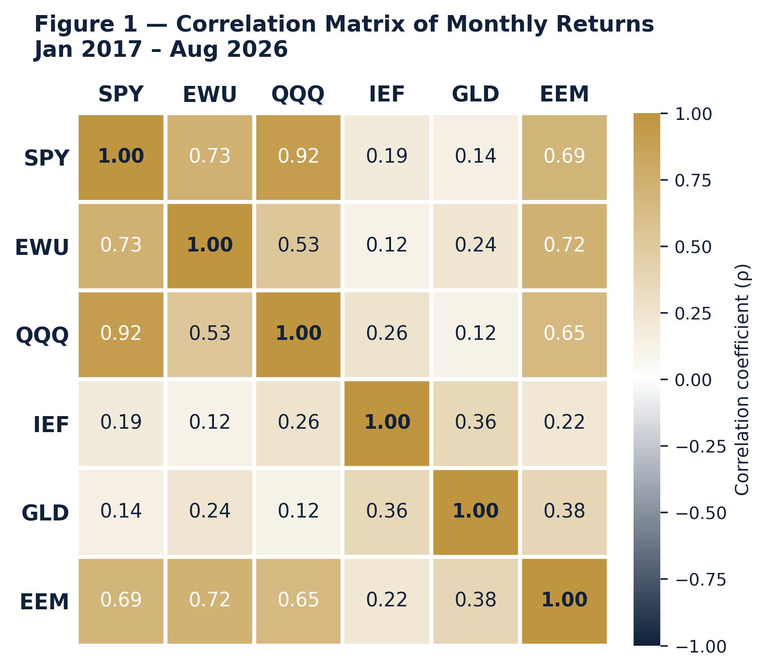
Figure 1 — Correlation matrix of monthly returns, Jan 2017 – Aug 2026.
Portfolio Construction
Portfolio variance is calculated exactly from the full covariance matrix:
Where w is the vector of portfolio weights and Σ is the covariance matrix.
And beta measures an asset's sensitivity to the broad market:
Sensitivity of asset i's returns to the market portfolio m.
Worked example — Portfolio A: σ²ₚ = (0.60)²(0.1553)² + (0.40)²(0.1928)² + 2(0.60)(0.40)(0.1553)(0.1928)(0.92) = 0.027853, so σₚ = √0.027853 = 16.69%.
Three portfolios were built from the same six ETFs to isolate whether holding count or correlation structure drives volatility:
| Portfolio | Weights | Return | Vol. (σₚ) | Sharpe | Avg. ρ |
|---|---|---|---|---|---|
| A — Concentrated | 60% SPY / 40% QQQ | 17.74% | 16.69% | 0.94 | 0.92 |
| B — "Diversified" equities | 25% each: SPY, EWU, QQQ, EEM | 13.71% | 14.99% | 0.78 | 0.71 |
| C — Cross-asset | 20% each: SPY, EWU, IEF, GLD, EEM | 9.84% | 10.49% | 0.75 | 0.38 |
A useful diagnostic for how much diversification a portfolio is actually achieving is the diversification ratio, DR = (Σᵢ wᵢσᵢ) / σₚ — the weighted-average volatility an investor would bear if every asset moved independently, divided by the volatility they actually bear. Portfolio A scores DR = 1.02 — essentially none. Portfolio B, with twice the holdings, only reaches DR = 1.13. Portfolio C, with one more holding than B, reaches DR = 1.34.
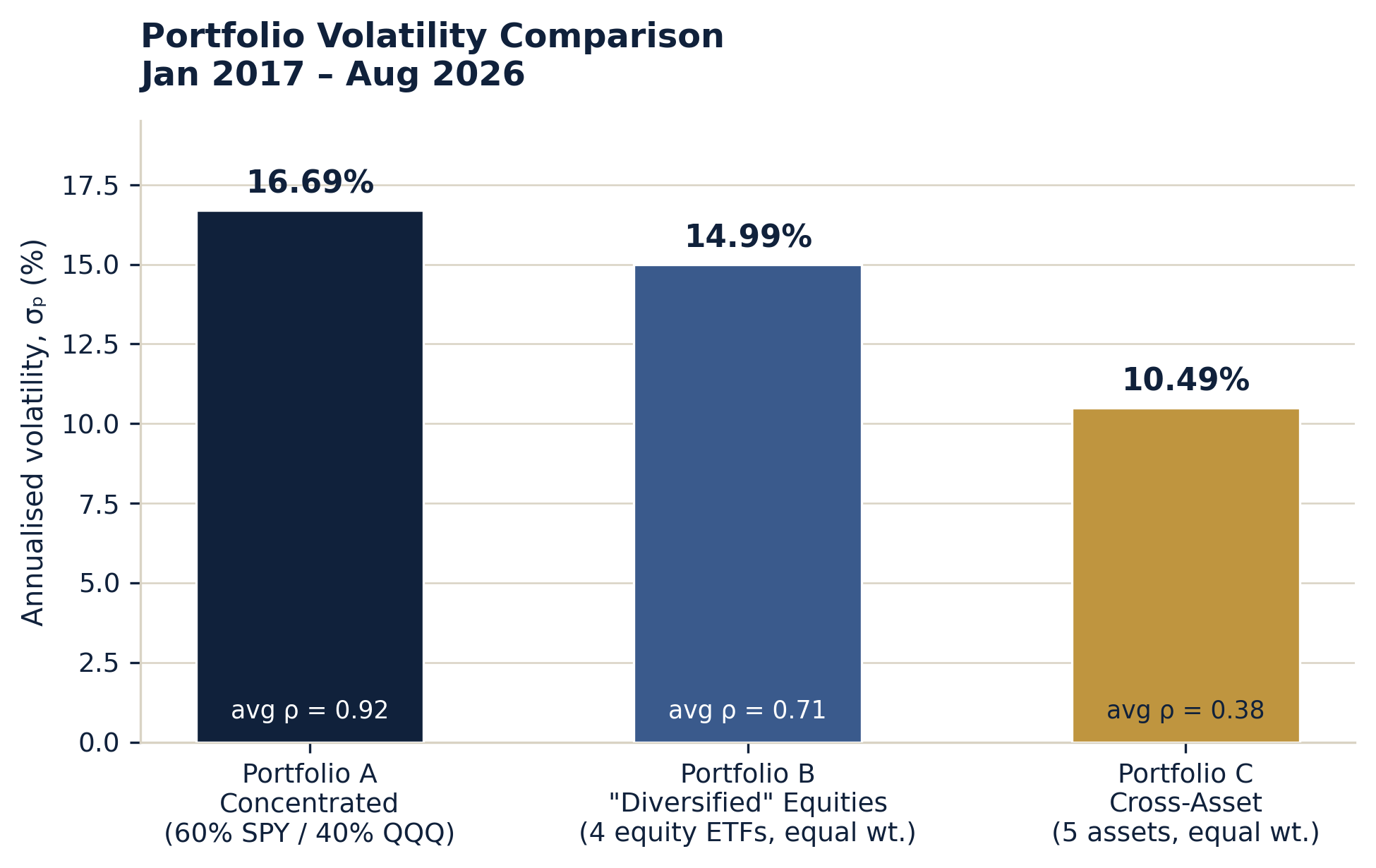
Figure 2 — Portfolio volatility comparison, Jan 2017 – Aug 2026.
Doubling the number of holdings (A → B) barely moves volatility, because every added name shares the same underlying equity risk factor (average pairwise ρ stays above 0.7). Adding a single bond-and-gold exposure (B → C) — one extra holding, not four — produces more than double the volatility reduction, because it lowers the average correlation of the book from 0.71 to 0.38.
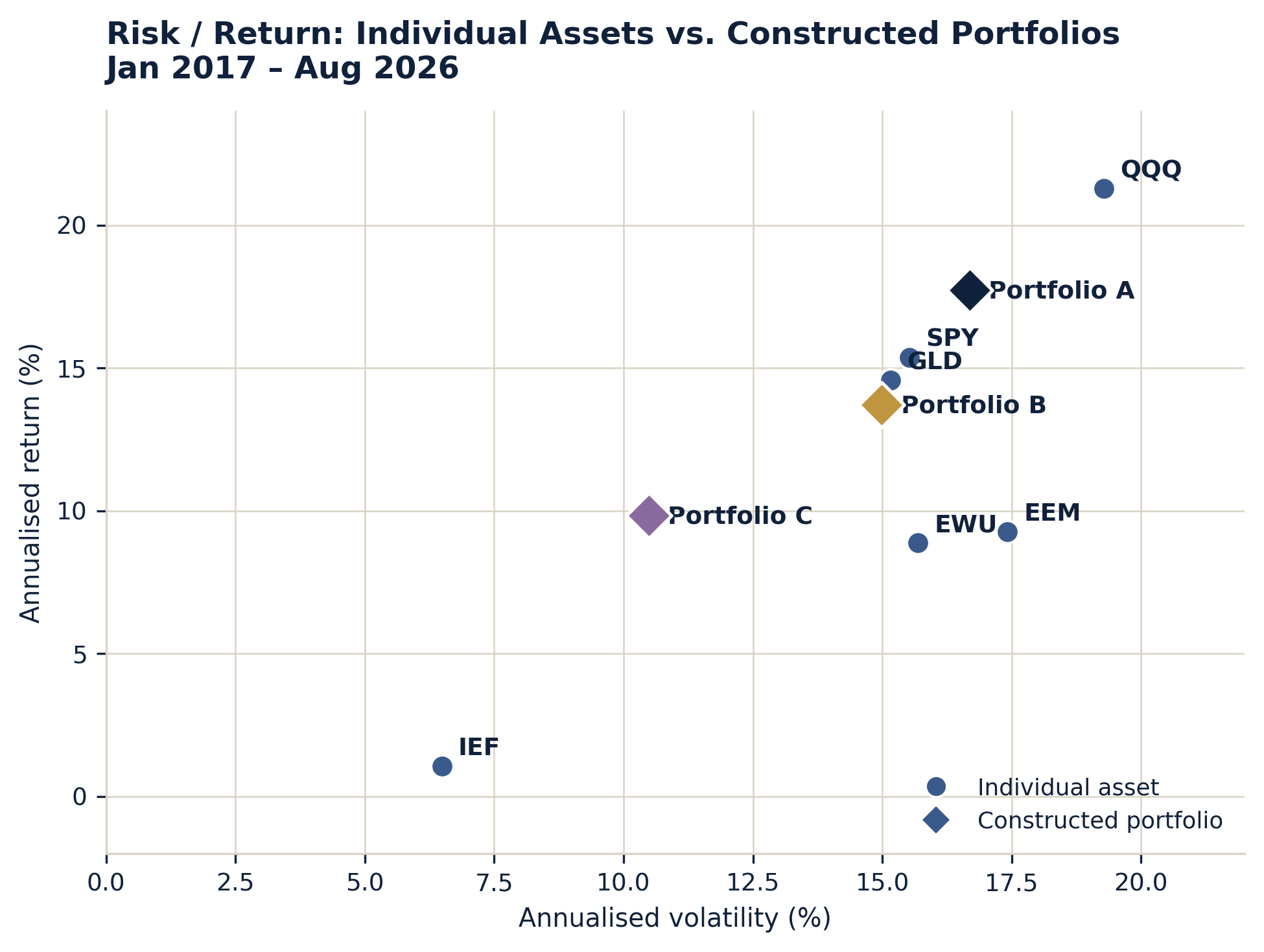
Figure 3 — Risk / return: individual assets vs. constructed portfolios.
Key Findings
Static, full-period correlations can mask what happens exactly when diversification is needed most. The sample was split into three regimes and the correlation matrix recomputed for each: the 2020 COVID crash, the 2022 rate-hike bear market, and 2023–25 as a calmer comparison window.
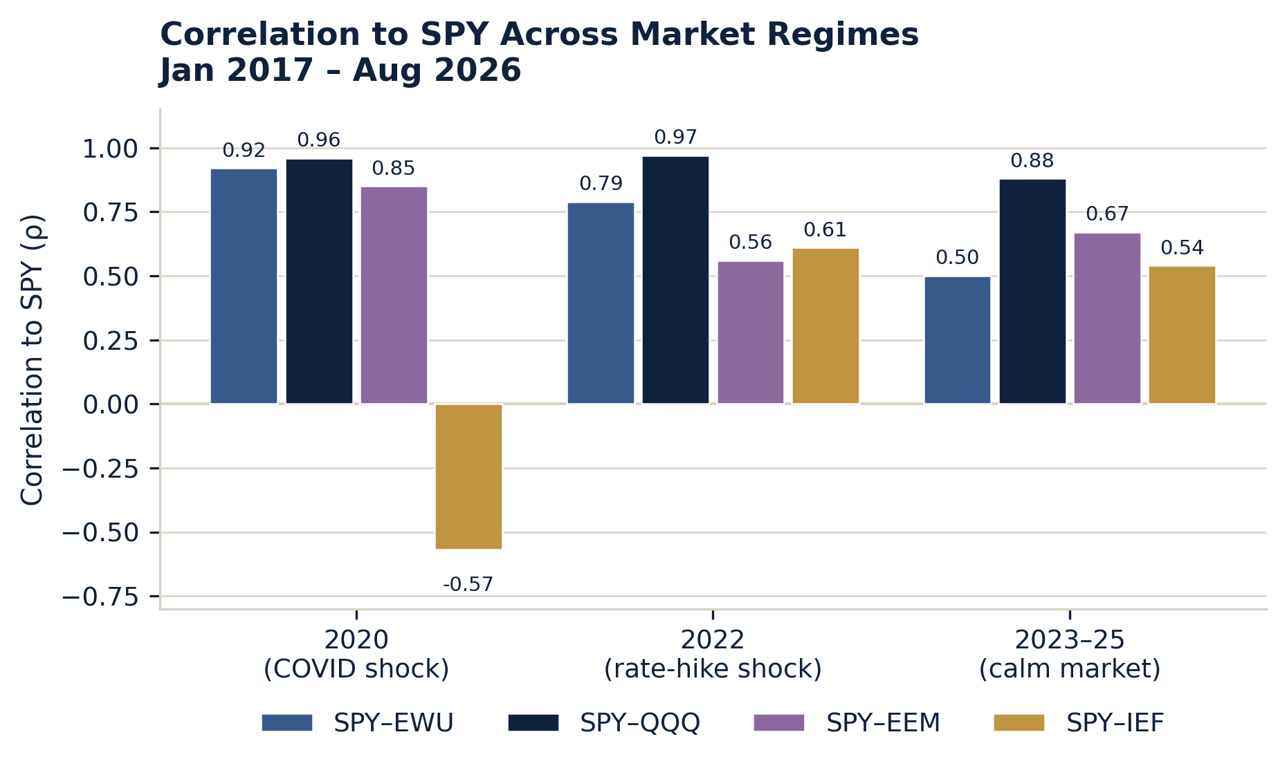
Figure 4 — Correlation to SPY across market regimes.
- Holding count is a weak predictor of diversification; correlation structure is the real one. Doubling equity holdings (Portfolio A → B) reduced volatility by only 1.7 points, because every added name shares the same underlying equity risk factor. Adding one cross-asset holding (B → C) reduced it by 4.5 points, because it lowered the average pairwise correlation from 0.71 to 0.38.
- Government bonds and gold provided the genuine diversification — not more equities. IEF and GLD were the only holdings with consistently low correlation to every equity in the set (ρ between 0.12 and 0.26), and carried the lowest betas (0.08 and 0.14). A second developed-market equity index (EWU) still correlated with SPY at ρ = 0.73.
- Which assets diversify a portfolio depends on the type of shock, not just its severity. Equity-to-equity correlations rose in both crisis windows relative to the calm 2023–25 period. But SPY–IEF (equity–bond) correlation moved in opposite directions: it fell to −0.57 in the 2020 growth/liquidity shock (bonds rallied as a flight-to-quality hedge while equities fell) and rose to +0.61 in the 2022 inflation/rate-hike shock (both asset classes were repriced by the same rising-discount-rate mechanism, so bonds fell alongside equities). A hedge that worked in the last crisis is not guaranteed to work in the next one if the next one has a different macroeconomic cause.
Limitations
- Portfolio-level returns are weight-averaged realised CAGRs rather than a full daily price-path backtest, so compounding/rebalancing drag on the return figure (not the volatility figure, which is exact) is only approximated; portfolio-level maximum drawdown was not computed for the same reason.
- Correlations are estimated on monthly returns; a daily-return matrix would likely show modestly different short-horizon correlations.
- The risk-free rate is a single backed-out approximation (≈2.0%) rather than a period-matched daily series.
- Historical correlations are not structural constants — as the stress-period analysis shows, they move with the macroeconomic regime, so the correlation matrix in Figure 1 describes 2017–2026, not a forecast.
- The choice of start date, ETF proxies, and USD-denominated returns (currency risk is not separated out for EWU or EEM) all affect the precise numbers reported here.
- Transaction costs, taxes, and rebalancing costs are excluded throughout.
None of this changes the central, structural result — correlation, not headcount, drives diversification — but all of it should temper how literally the specific percentages are read.
Conclusion
Across three portfolios built from the same six building blocks, the number of holdings explained very little of the realised volatility difference; average pairwise correlation explained almost all of it. Doubling equity holdings (Portfolio A → B) reduced volatility by 1.7 points; adding one cross-asset holding (B → C) reduced it by 4.5 points. The stress-period analysis adds a second layer: even the "good" diversifiers are regime-dependent — government bonds hedged the 2020 shock and failed to hedge the 2022 shock, because the two crises had different macroeconomic drivers.
Read the complete methodology, figures and analysis in the full paper.
Download Full Research Paper